Introduction to Mechanistic Interpretability, Superposition and Sparse Autoencoders
In this post, we will explore the concepts of Superposition and Sparse Autoencoders in the context of mechanistic interpretability. We'll build a spar...
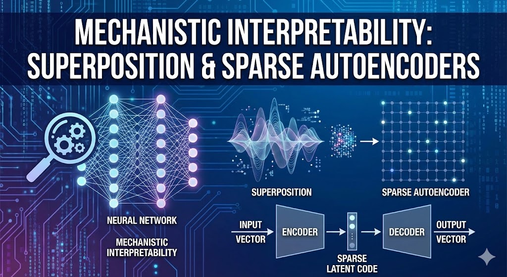
In this post, we will explore the concepts of Superposition and Sparse Autoencoders in the context of mechanistic interpretability. We’ll build a sparse autoencoder from scratch and use it to decompose the activations of a pre-trained transformer model.
Mechanistic Interpretability
The goal of mechanistic intepretability is to be able to reverse engineer a neural network model to not just understand what predictions it makes, but also how it arrives to those predictions through internal computational mechanism.
Why does this matter? Consider a languaguge model that refuses to answer a sensitive topic e.g. (b0mb making). Is it refusing because it has learned a general principle of “don’t help with dangerous requests?” or it has simply memorized a list of banned keywords? The difference is very critical for AI safety. The first model might generalize well to novel dangerous requests, while the second might be trivially jailbroken with synonym substitution or mildly complex rephrasing of the request. Without understanding the underlying mechanism, we are kind of flying blind.
Mechanistic Interpretability goes beyond the correlation based approaches (like “this neuron activates for past tense”) to ask causal questions: *What computation is this circuit performing? What algorithm has the model learned? For example, we might discover that a tranformer implements an induction head. It is a circuit that predicts repeated tokens by matching patterns like “P Q…P -> Q”. This is a mechanistic explanation. We can tracte the information flow through attention heads, show how earlier heads move information and later heads use it, and even predict when the circuit will fire.
This approach gives us a shot at understanding whether models have learned the “right” algorithms for the right reasons, which is essential for building systems we can trust at scale. It is also deeply connected to AI alignment, if we can’t explain how a model really works, how can we be confident it will behave safely in a novel situation?
Path Decomposition of transformer output
A transformer model’s operations can be broken down into many different “paths” the information can flow through. This is mostly due to presence of residual connection in the model. Residual connections allows model to be an ensemble of many models. If a model has $n$ layers, there are essentially $2^n$ possible paths for the information to flow. This concept allows you to take a specific operation within the transformer and break it down into the various paths information could have traveled through the model to achieve that operation. If we have single layer of transformer, then information flow can only have two paths:
Direct Path (embedding and unembedding):This is the simplest path where the input tokens are embedded and then directly unembedded. In a transformer with only embedding and unembedding, the model can primarily learn bigram frequency statistics. This means it can only condition on the previous token, similar to a Markovian model.
Path Through the Layer (embedding → layer → unembedding): This path passes through the actual transformer layer. The attention mechanism allows the model to move information between token positions, enabling it to look at context beyond just the previous token. The MLP sublayer then performs nonlinear transformations on the attended representations. This path is where the model develops more sophisticated capabilities beyond simple bigram statistics. It can implement circuits for tasks like induction (copying previous patterns), indirect object identification, or tracking subject-verb agreement across long distances.
This leads to concept of circuit.
Circuit
A circuit is defined as subgraph of the transformer that represents the specific path a model uses to perform a particular task. By identifying these circuits, researchers can gain causal evidence of how the transformer accompalishes a certain taks. If ablating components along a critical path causes the model to fail at the task, it strongly suggests that path is the mechanism used by transformer.
Residual stream as output accumulation
Another concept in the mechanistic intepretability is residual stream. The residual stream is the central information highway in a transformer. It’s the sequence of vector representations that flows throught the model., which each component (attention heads, MLP layers) reading from it and writing back to it. Think of this residual stream as the running accumulation of the information. At the start, it contains just the token embeddings. Then each component adds its contribution.
\[\text{residual}_{\text{layer } n} = \text{residual}_{\text{layer } n-1} + \text{attention}_{n} + \text{MLP}_{n}\]Each attention head and MLP layer reads the current residual stream, performs its computation, and writes its output back into the residual stream via the residual connection. The final prediction is computed by taking the last residual stream vector at each position and projecting it through the unembedding matrix.
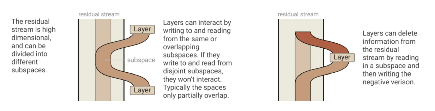
The residual view reveals that transformers work by iterative refinement. Early layers might identify basic features (“this is a noun”), middle layers might compose these into relationships (“this noun is the subject”), and later layers might use that context for the final prediction. Each layer adds a “correction” or “update” to the accumulated information.
This also explains why transformers can implement so many paths. Each component can independently contribute to the final output. Some paths might be dominant for certain inputs (e.g., the direct path for simple bigram predictions), while complex reasoning might require contributions from many layers working together.
Superposition
Now imagine you have a trained transformer model, where each individual neuron maps to a distinct, human interpretable feature of the text. For e.g. neural 56 in layer 3 fires for past-tense verbs. Similarly another neuron fires for location and another for negative sentiment. That would be be ideal case for Mechanistic Interpretability, a clean 1:1 correspondence between neuron and human understandable concepts. This happens once in a while however it is quite rare especially when models scale up. In large language models, most of the neurons don’t correspond to anything which we can easily describe. They active in a messy, polysemantic ways often firing for multiple unrelated features or forming features through combinations of many neurons working together. This is what we call Superposition.
Superposition is when model represents more than $n$ features in an $n$-dimensional activation space. The features still corresponds to direction in activation space but the set of interpretable directionsis larger than the number of dimension - Neel Nanda
Think of it this way, a model with 1,000 neurons theoretically has 1,000 dimensions to work with, but the world contains far more than 1,000 meaningful features. Natural language involves tens of thousands of concepts from concrete nouns to abstract grammatical structures to contextual nuances. How can a model represent all these features with so few neurons? The answer is superposition. Models learn to pack multiple features into the same set of neurons by exploiting sparsity. Most features are zero most of the time you don’t talk about duck in most sentences, for instance. By carefully arranging features as directions in activation space (not aligned with individual neurons), models can represent far more features than they have dimensions, at the cost of interference between features when multiple activate simultaneously.
Think of it like a compression algorithm: you’re storing more information than you have space for, accepting some loss of fidelity in exchange for greater capacity. This explains why neurons appear polysemantic : a single neuron participates in representing many different feature directions. It also explains why interpretability is so hard: the features we care about aren’t neatly aligned with the model’s physical architecture. They’re encoded in complex, overlapping patterns across many neurons. This creates a core challenge for AI safety: if we can’t cleanly identify what features a model has learned, how can we ensure it’s learned the right ones? How do we detect deceptive or dangerous capabilities hiding in superposition?
Sparse Autoencoders
What if we could decompress this compressed information? This is exactly what Sparse Autoencoders (SAEs) are designed to do.
The core insight is elegant: if the model is storing features in superposition by exploiting sparsity, we can try to reverse this compression by training an autoencoder that explicitly encourages sparse representations. The autoencoder learns to map the model’s dense, polysemantic activations into a higher-dimensional space where features are more clearly separated.
Architecture
A sparse autoencoder consists of two parts:
Encoder: Maps the model’s activations into a larger, sparse feature space
\[f_{\text{enc}}(x) = \text{ReLU}(W_{\text{enc}} x + b_{\text{enc}})\]Decoder: Reconstructs the original activations from the sparse features
\[f_{\text{dec}}(f) = W_{\text{dec}} f + b_{\text{dec}}\]
The key architectural choice is that the encoder output is overcomplete. It has many more dimensions than the input. For example, if we’re analyzing activations from a layer with 2,048 neurons, we might use an SAE with 16,384 or even 65,536 features. This overcomplete representation gives us room to spread out the compressed features that were packed together in superposition.
Training Objective
The SAE is trained with two competing objectives:
Reconstruction loss: The output should closely match the input activations
\[\mathcal{L}_{\text{recon}} = \|x - f_{\text{dec}}(f_{\text{enc}}(x))\|^2\]Sparsity penalty: The encoded features should be sparse (mostly zero)
\[\mathcal{L}_{\text{sparse}} = \lambda \|f_{\text{enc}}(x)\|_1\]
The total loss combines both:
\[\mathcal{L} = \mathcal{L}_{\text{recon}} + \mathcal{L}_{\text{sparse}}\]The L1 penalty ($|\cdot|_1$, sum of absolute values) encourages the encoder to activate as few features as possible to reconstruct the input. This forces the SAE to learn a sparse decomposition where each feature corresponds to a specific, interpretable concept.
Why This Works
The SAE is essentially learning to undo the compression the transformer performed. Because we’re training on the actual activations from a trained model, the SAE learns to decompose them in a way that respects the structure the model has already learned. The sparsity constraint forces it to find features that are genuinely sparse in the data—which are exactly the kinds of features the model likely learned to exploit for superposition in the first place.
When it works well, each SAE feature corresponds to a single interpretable concept. For example, in a trained SAE on GPT-2, researchers have found features that cleanly activate for:
- Base64 encoded text
- Specific programming languages (Python vs. JavaScript)
- References to particular cities or countries
- Grammatical structures like indirect objects
- Abstract concepts like “items in a list”
These features often activate much more cleanly than individual neurons, giving us a window into the model’s internal representations.
Think of it like this:
- Input: Dense 768-d activation (many features compressed)
- SAE encoder: Finds which features are present
- Sparse code: Only ~10-50 features active (interpretable!)
- SAE decoder: Reconstructs the original from these features
Step1: Setup and Imports
1
2
3
4
5
6
7
!pip install -q transformer_lens
!pip install -q einops
!pip install -q plotly
!pip install -q circuitsvis
!pip install -q pandas
!pip install -q datasets
1
2
3
4
5
6
7
8
9
10
11
12
13
14
15
16
17
18
19
20
21
22
23
24
25
import torch
import torch.nn as nn
import torch.nn.functional as F
from torch.utils.data import Dataset, DataLoader
import numpy as np
import pandas as pd
import einops
from tqdm.auto import tqdm
import plotly.express as px
import plotly.graph_objects as go
import IPython.display # Added this line
from plotly.subplots import make_subplots # Added this line

from dataclasses import dataclass
from typing import Tuple
from pprint import pprint


from transformer_lens import HookedTransformer
from datasets import load_dataset

device = 'cuda' if torch.cuda.is_available() else 'cpu'

torch.manual_seed(123)
np.random.seed(42)
Step 2: Implementing the Sparse Autoencoder
We’ll implement our SAE from scratch. We’ll include, the core architecture, training code and feature analysis.
1
2
3
4
5
6
7
8
9
10
11
12
@dataclass
class SAEConfig:
  """Configuration for Sparse AutoEncoder"""
  d_model: int = 768  # Input dimension e.g. GPT-2 residual stream size
  expansion_factor: int = 8 #Hidden layer expansion (d_hiddn = expansion_factor * d_model)
  lambda_sparse: float = 1e-3 #sparsity penalty coefficient
  learning_rate: float = 1e-3 #learning rate for training

  @property
  def d_hidden(self) -> int:
    return self.d_model * self.expansion_factor
1
2
cfg = SAEConfig()
pprint(cfg, indent=2)
1
2
3
4
SAEConfig(d_model=768,
          expansion_factor=8,
          lambda_sparse=0.001,
          learning_rate=0.001)
1
2
3
4
5
6
7
8
9
10
11
12
13
14
15
16
17
18
19
20
21
22
23
24
25
26
27
28
29
30
31
32
33
34
35
36
37
38
39
40
41
42
43
44
45
46
47
48
49
50
51
52
53
54
55
56
57
58
59
60
61
62
63
64
65
66
67
68
69
70
71
72
73
74
75
76
77
78
79
80
81
82
83
84
85
86
87
88
89
90
91
class SparseAutoEncoder(nn.Module):
  def __init__(self, cfg: SAEConfig):
    super().__init__()
    self.cfg = cfg

    # Encoder: d_model -> d_hidden
    self.W_enc = nn.Parameter(torch.randn(cfg.d_hidden, cfg.d_model) / np.sqrt(cfg.d_model))
    self.b_enc = nn.Parameter(torch.zeros(cfg.d_hidden))


    # Decoder: d_hideen -> d_model
    self.W_dec = nn.Parameter(torch.randn(cfg.d_model, cfg.d_hidden) / np.sqrt(cfg.d_hidden))
    self.b_dec = nn.Parameter(torch.zeros(cfg.d_model))


    # Initialize decoder columns to unit norm
    # This helps with training stability
    self.W_dec.data = self.W_dec.data / self.W_dec.data.norm(dim=0, keepdim=True)


  def encode(self, x: torch.Tensor) -> torch.Tensor:
    """Encode input to sparsee feature representation
    Args:
      x: Input activations [batch, d_model]

    Returns:
      f: Sparse features [batch, d_hidden]
    """
    x_centered = x - self.b_dec
    pre_activation = x_centered @ self.W_enc.T + self.b_enc
    f = F.relu(pre_activation)
    return f


  def decode(self, f: torch.Tensor) -> torch.Tensor:
    """Decode sparse feature back into the activation space.
    Args:
      f: Sparce features [batch, d_hidden]

    Returns:
      x_reconstructed: Reconstructed activations [batch d_model]
    """
    x_reconstructed = f @ self.W_dec.T + self.b_dec
    return x_reconstructed

  def forward(self, x: torch.Tensor) -> Tuple[torch.Tensor, torch.Tensor]:
    """
    Forward pass: encode and decode
    Args:
      x: Input activations [batch, d_model]
    Returns:
      x_reconstructed: Reconstructed Activations [batch, d_model]
      f: sparse feature activations [batch, d_hidden]
    """
    f = self.encode(x)
    x_reconstructed = self.decode(f)

    return x_reconstructed, f

  def compute_loss(self, x: torch.Tensor) -> Tuple[torch.Tensor, dict]:
    """
    Compute reconstruction loss + sparsity penalty

    Args:
      x: Input Activations [batch, d_mdoel]

    Returns:
      total_loss: combined loss (reconstruction + sparsity)
      metrics: Dict of metrics for logging
    """
    x_reconstructed, f = self.forward(x)

    # reconstruction loss: MSE
    reconstruction_loss = (x - x_reconstructed).pow(2).mean()

    # sparsity penalty
    sparsity_loss = f.abs().sum(dim=-1).mean()
    total_loss = reconstruction_loss + self.cfg.lambda_sparse * sparsity_loss

    l0_norm = (f > 0).float().sum(dim=-1).mean() #avg number of active features
    metrics = {
        'loss': total_loss.item(),
        'reconstruction_loss': reconstruction_loss.item(),
        'sparsity_loss': sparsity_loss.item(),
        'l0_norm': l0_norm.item()
    }

    return total_loss, metrics
1
2
3
4
5
6
sae = SparseAutoEncoder(cfg).to(device)

print(f"SAE Architecture")
print(f"  Parameters: {sum(p.numel() for p in sae.parameters())}")
print(f"  Encoder: {cfg.d_model} -> {cfg.d_hidden}")
print(f"  Decoder: {cfg.d_hidden} -> {cfg.d_model}")
1
2
3
4
SAE Architecture
  Parameters: 9444096
  Encoder: 768 -> 6144
  Decoder: 6144 -> 768
Step 3: Testing
Let’s test with some random input to make sure our training loop works as expected and we can calculate loss.
1
2
3
4
5
6
7
8
9
10
11
12
13
14
15
16
17
x_test = torch.randn(32, cfg.d_model).to(device)

x_recon, f = sae(x_test)

print(f"Input shape: {x_test.shape}")
print(f"Features shape: {f.shape}")
print(f"Reconstruction shape: {x_recon.shape}")
print(f"\nFeature statistics:")
print(f"  Active features: {(f > 0).float().sum(dim=-1).mean().item():.1f} / {cfg.d_hidden}")
print(f"  Sparsity: {100 * (f > 0).float().mean().item():.2f}% of features active")

# Compute loss
loss, metrics = sae.compute_loss(x_test)
print(f"\nLoss components:")
for k, v in metrics.items():
    print(f"  {k}: {v:.6f}")
1
2
3
4
5
6
7
8
9
10
11
12
13
Input shape: torch.Size([32, 768])
Features shape: torch.Size([32, 6144])
Reconstruction shape: torch.Size([32, 768])

Feature statistics:
  Active features: 3081.2 / 6144
  Sparsity: 50.15% of features active

Loss components:
  loss: 7.526083
  reconstruction_loss: 5.069376
  sparsity_loss: 2456.707520
  l0_norm: 3081.187500
Part 4: Collecting Activation Data from GPT-2
To train our SAE, we need activation data from a real model. We’ll:
- Load GPT-2 Small
- Run text through it
- Extract activations from a specific layer (e.g., the MLP output of layer 6)
- Store these activations as our training data
Why Layer 6?
Middle layers tend to contain the most interesting features because usually the first few layers are low level features like tokens and the last few layers are task specific features like next token prediction. The middle layers are where the model learns the most interesting features.
We’ll use layer 6 (middle of the 12 layers) to find interesting semantic features.
1
2
3
4
5
6
7
8
9
10
11
model = HookedTransformer.from_pretrained(
    "gpt2-small",
    device=device
)


print(f"Loaded GPT-2 Small:")
print(f"  Layers: {model.cfg.n_layers}")
print(f"  Hidden size: {model.cfg.d_model}")
print(f"  Vocabulary: {model.cfg.d_vocab}")
1
2
3
4
5
Loaded pretrained model gpt2-small into HookedTransformer
Loaded GPT-2 Small:
  Layers: 12
  Hidden size: 768
  Vocabulary: 50257
1
2
3
4
# load a dataset
dataset = load_dataset("ag_news", split="train[:10%]")  # small slice
print(f"Total examples: {len(dataset)}")
1
dataset[123]
1
2
{'text': 'Appeal Rejected in Trout Restoration Plan (AP) AP - The U.S. Forest Service on Wednesday rejected environmentalists\' appeal of a plan to poison a stream south of Lake Tahoe to aid what wildlife officials call "the rarest trout in America."',
 'label': 3}
1
2
3
4
5
6
7
8
9
10
# A simple Dataset to yield raw texts for batching
class TextDataset(Dataset):
  def __init__(self, hf_dataset):
    self.hf_dataset = hf_dataset

  def __len__(self):
    return len(self.hf_dataset)

  def __getitem__(self, idx):
    return self.hf_dataset[idx]['text']
1
2
3
4
5
6
7
8
9
10
11
12
13
14
15
16
17
18
19
20
21
22
23
24
25
26
27
28
29
30
31
def collect_activations(model: HookedTransformer, dataset: Dataset, layer_idx: int = 6, hook_point: str = "mlp_out", batch_size: int = 32) -> torch.Tensor:
  """
  Collect activations from a specific layer and hook point, processing in batches.
  Args:
    model: HookedTransformer model
    dataset: dataset containing the text
    layer_idx: which layer to extract from
    hook_point: Which activation to extract (e.g. "mlp_out", "resid_post")
    batch_size: Number of examples to process in each batch.

  Returns:
    activations: Tensor of shape [n_total_tokens, d_model]
  """
  all_activations = []
  hook_name = f"blocks.{layer_idx}.hook_{hook_point}"

  # Create a DataLoader to batch the text examples
  text_dataset_for_batching = TextDataset(dataset) # Use the new TextDataset
  dataloader = DataLoader(text_dataset_for_batching, batch_size=batch_size, shuffle=False)

  for batch_of_texts in tqdm(dataloader, desc=f"Collecting activations from layer {layer_idx} (batched)"):
    # model.to_tokens can take a list of strings and will tokenize/pad them
    tokens = model.to_tokens(batch_of_texts).to(device)
    _, cache = model.run_with_cache(tokens)
    acts = cache[hook_name]

    # Flatten the activations from [batch_size, seq_len, d_model] to [total_tokens_in_batch, d_model]
    all_activations.append(acts.view(-1, acts.shape[-1]))

  activations = torch.cat(all_activations, dim=0)
  return activations
1
2
3
print("Collecting activations from GPT-2...")
activations = collect_activations(model, dataset, layer_idx=6, batch_size=32)
print(f"Collected activations shape: {activations.shape}")
1
2
3
4
5
6
7
8
Collecting activations from GPT-2...


Collecting activations from layer 6 (batched):   0%|          | 0/375 [00:00<?, ?it/s]


Collected activations shape: torch.Size([1348480, 768])
An activation pytorch dataset
We’ll wrap our activations in a Pytorch Dataset for efficient batching during training.
1
2
torch.save(activations, "gpt2_mlp_out_activations_layer6.pt")
print("Activations saved to gpt2_mlp_out_activations_layer6.pt")
1
Activations saved to gpt2_mlp_out_activations_layer6.pt
1
2
3
4
5
6
7
8
9
10
11
12
13
14
15
16
17
18
19
20
21
22
23
24
25
class ActivationDataset(Dataset):
    """Dataset of neural network activations"""

    def __init__(self, activations: torch.Tensor):
        self.activations = activations

    def __len__(self):
        return len(self.activations)

    def __getitem__(self, idx):
        return self.activations[idx]

# Create dataset and dataloader
dataset = ActivationDataset(activations)
dataloader = DataLoader(
    dataset,
    batch_size=256,
    shuffle=True,
    pin_memory=False
)

print(f"Dataset created:")
print(f"  Total samples: {len(dataset):,}")
print(f"  Batches per epoch: {len(dataloader)}")
print(f"  Batch size: 256")
1
2
3
4
Dataset created:
  Total samples: 1,348,480
  Batches per epoch: 5268
  Batch size: 256
1
2
3
4
5
6
7
8
9
10
11
12
13
14
15
16
17
18
19
20
21
22
23
24
25
26
27
28
29
30
31
32
33
34
35
36
37
38
39
40
41
42
43
44
45
46
47
48
49
50
51
52
53
54
55
56
57
58
59
60
61
62
63
64
65
66
67
68
69
70
def train_sae(sae, dataloader, n_epochs=10, device='cuda'):
    """
    Train the Sparse Autoencoder.

    Args:
        sae: SparseAutoencoder model
        dataloader: DataLoader with activation data
        n_epochs: Number of training epochs
        device: Device to train on

    Returns:
        history: Dictionary of training metrics
    """
    # Set up optimizer
    optimizer = torch.optim.Adam(sae.parameters(), lr=sae.cfg.learning_rate)

    # Training history
    history = {
        'loss': [],
        'reconstruction_loss': [],
        'sparsity_loss': [],
        'l0_norm': []
    }

    sae.train()

    for epoch in range(n_epochs):
        epoch_metrics = {k: [] for k in history.keys()}

        pbar = tqdm(dataloader, desc=f"Epoch {epoch+1}/{n_epochs}")

        for batch in pbar:
            batch = batch.to(device)

            # Zero gradients
            optimizer.zero_grad()

            # Forward pass and compute loss
            loss, metrics = sae.compute_loss(batch)

            # Backward pass
            loss.backward()

            # Update weights
            optimizer.step()

            # Normalize decoder columns (keeps training stable)
            with torch.no_grad():
                sae.W_dec.data = sae.W_dec.data / sae.W_dec.data.norm(dim=0, keepdim=True)

            # Track metrics
            for k, v in metrics.items():
                epoch_metrics[k].append(v)

            # Update progress bar
            pbar.set_postfix({
                'loss': f"{metrics['loss']:.4f}",
                'L0': f"{metrics['l0_norm']:.1f}"
            })

        # Average metrics for the epoch
        for k in history.keys():
            history[k].append(np.mean(epoch_metrics[k]))

        print(f"Epoch {epoch+1} - Loss: {history['loss'][-1]:.4f}, "
              f"Recon: {history['reconstruction_loss'][-1]:.4f}, "
              f"L0: {history['l0_norm'][-1]:.1f}")

    return history
1
2
3
4

# Train the SAE
print("Training Sparse Autoencoder...\n")
history = train_sae(sae, dataloader, n_epochs=12, device=device)
1
2
3
4
5
6
7
8
9
10
11
12
13
14
15
16
17
18
19
20
21
22
23
24
25
26
27
28
29
30
31
32
33
34
35
36
37
38
39
40
41
42
43
44
45
46
47
48
49
50
51
52
53
54
55
56
57
58
59
60
61
62
63
64
65
66
67
68
69
70
71
72
73
74
75
76
77
78
79
80
81
82
83
84
85
86
Training Sparse Autoencoder...


Epoch 1/12:   0%|          | 0/5268 [00:00<?, ?it/s]


Epoch 1 - Loss: 0.1750, Recon: 0.1009, L0: 141.3


Epoch 2/12:   0%|          | 0/5268 [00:00<?, ?it/s]


Epoch 2 - Loss: 0.1326, Recon: 0.0730, L0: 117.4


Epoch 3/12:   0%|          | 0/5268 [00:00<?, ?it/s]


Epoch 3 - Loss: 0.1255, Recon: 0.0700, L0: 109.2


Epoch 4/12:   0%|          | 0/5268 [00:00<?, ?it/s]


Epoch 4 - Loss: 0.1233, Recon: 0.0688, L0: 105.2


Epoch 5/12:   0%|          | 0/5268 [00:00<?, ?it/s]


Epoch 5 - Loss: 0.1225, Recon: 0.0684, L0: 103.2


Epoch 6/12:   0%|          | 0/5268 [00:00<?, ?it/s]


Epoch 6 - Loss: 0.1221, Recon: 0.0681, L0: 102.3


Epoch 7/12:   0%|          | 0/5268 [00:00<?, ?it/s]


Epoch 7 - Loss: 0.1218, Recon: 0.0679, L0: 101.6


Epoch 8/12:   0%|          | 0/5268 [00:00<?, ?it/s]


Epoch 8 - Loss: 0.1216, Recon: 0.0677, L0: 101.4


Epoch 9/12:   0%|          | 0/5268 [00:00<?, ?it/s]


Epoch 9 - Loss: 0.1215, Recon: 0.0677, L0: 100.8


Epoch 10/12:   0%|          | 0/5268 [00:00<?, ?it/s]


Epoch 10 - Loss: 0.1214, Recon: 0.0677, L0: 100.8


Epoch 11/12:   0%|          | 0/5268 [00:00<?, ?it/s]


Epoch 11 - Loss: 0.1213, Recon: 0.0676, L0: 100.5


Epoch 12/12:   0%|          | 0/5268 [00:00<?, ?it/s]


Epoch 12 - Loss: 0.1212, Recon: 0.0676, L0: 100.4
1
2
3
4
# Save the SAE model's state dictionary
model_save_path = "sae_model_state_dict.pth"
torch.save(sae.state_dict(), model_save_path)
print(f"SAE model state dictionary saved to {model_save_path}")
1
SAE model state dictionary saved to sae_model_state_dict.pth
1
2
3
4
5
6
7
8
9
10
11
12
13
14
15
16
# Load the SAE model's state dictionary
model_load_path = "sae_model_state_dict.pth"

# Create a new SAE instance with the same configuration
loaded_sae = SparseAutoEncoder(cfg).to(device)

# Load the state dictionary
loaded_sae.load_state_dict(torch.load(model_load_path))
loaded_sae.eval() # Set to evaluation mode

print(f"SAE model loaded from {model_load_path}")

# Optional: Verify by running a quick forward pass
x_test_load = torch.randn(32, cfg.d_model).to(device)
x_recon_load, f_load = loaded_sae(x_test_load)
print(f"Loaded SAE: Features shape: {f_load.shape}, Reconstruction shape: {x_recon_load.shape}")
1
2
SAE model loaded from sae_model_state_dict.pth
Loaded SAE: Features shape: torch.Size([32, 6144]), Reconstruction shape: torch.Size([32, 768])
1
2
3
4
5
6
7
8
9
10
11
12
13
14
15
16
17
18
19
20
21
22
23
24
25
26
27
28
29
30
31
32
33
34
35
36
37
38
39
40
41
42
43
44
45
46
47
48
49
50
51
52
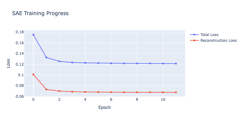
# Plot training curves
import IPython.display
fig = go.Figure()
fig.add_trace(go.Scatter(
y=history['loss'],
name='Total Loss',
mode='lines+markers'
))
fig.add_trace(go.Scatter(
y=history['reconstruction_loss'],
name='Reconstruction Loss',
mode='lines+markers'
))
fig.update_layout(
title="SAE Training Progress",
xaxis_title="Epoch",
yaxis_title="Loss",
width=800,
height=400
)
IPython.display.display(fig)
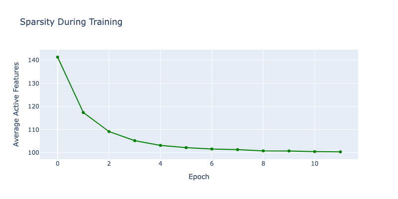
# Plot sparsity
fig2 = go.Figure()
fig2.add_trace(go.Scatter(
y=history['l0_norm'],
name='Active Features (L0)',
mode='lines+markers',
line=dict(color='green')
))
fig2.update_layout(
title="Sparsity During Training",
xaxis_title="Epoch",
yaxis_title="Average Active Features",
width=800,
height=400
)
IPython.display.display(fig2)
print(f"\nFinal metrics:")
print(f" Total loss: {history['loss'][-1]:.4f}")
print(f" Reconstruction loss: {history['reconstruction_loss'][-1]:.4f}")
print(f" Active features: {history['l0_norm'][-1]:.1f} / {cfg.d_hidden}")
print(f" Sparsity: {100 * history['l0_norm'][-1] / cfg.d_hidden:.2f}%")
1
2
3
4
5
Final metrics:
  Total loss: 0.1212
  Reconstruction loss: 0.0676
  Active features: 100.4 / 6144
  Sparsity: 1.63%
Part 6: Analyzing Learned Features
Now comes the exciting part: what did our SAE learn? Let’s analyze the features it discovered.
What to Look For
Good SAE features should:
- Be interpretable: Activate for clear, understandable patterns
- Be specific: Activate for one concept, not a mix
- Be sparse: Only a few features active at once
- Reconstruct well: Preserve the original information
1
2
3
4
5
6
7
8
9
10
11
12
13
14
15
16
17
18
19
20
21
22
23
24
25
26
27
28
29
30
31
32
33
34
35
36
37
38
39
40
41
42
43
44
45
46
47
48
49
50
51
52
53
54
55
56
57
58
59
60
def analyze_feature_activations(sae, texts, model, layer_idx=6, top_k=10):
    """
    Analyze which features activate most for given texts.

    Args:
        sae: Trained SparseAutoencoder
        texts: List of texts to analyze
        model: Language model
        layer_idx: Which layer to extract from
        top_k: Number of top features to return per text

    Returns:
        results: List of (text, top_features, top_values)
    """
    sae.eval()
    results = []

    hook_name = f"blocks.{layer_idx}.hook_mlp_out"

    with torch.no_grad():
        for text in texts:
            # Get activations
            tokens = model.to_tokens(text)
            _, cache = model.run_with_cache(tokens)
            acts = cache[hook_name].squeeze(0)  # [seq_len, d_model]

            # Encode to features
            features = sae.encode(acts.to(device))  # [seq_len, d_hidden]

            # Average over sequence
            avg_features = features.mean(dim=0)  # [d_hidden]

            # Get top activating features
            top_values, top_indices = torch.topk(avg_features, top_k)

            results.append({
                'text': text,
                'top_features': top_indices.cpu().numpy(),
                'top_values': top_values.cpu().numpy()
            })

    return results

# Analyze some test texts
test_texts = [
    "The capital of France is Paris.",
    "The MSFT stock shows most promising quarter",
    "The sun rises in the east.",
    "The financial markets largely reacted positive to the news.",
]

print("Analyzing feature activations...\n")
results = analyze_feature_activations(sae, test_texts, model)

for r in results:
    print(f"Text: '{r['text']}'")
    print(f"Top features: {r['top_features']}")
    print(f"Activation values: {r['top_values']}")
    print()
1
2
3
4
5
6
7
8
9
10
11
12
13
14
15
16
17
18
19
20
21
Analyzing feature activations...

Text: 'The capital of France is Paris.'
Top features: [1123 4656 4906 5045 5728 2829 1077 5014 4698 3669]
Activation values: [7.5884004  3.7092948  2.3116324  1.2506702  1.0750544  1.0149817
 0.96417254 0.9448468  0.8581832  0.80127203]

Text: 'The MSFT stock shows most promising quarter'
Top features: [1123 4906 5217 4656 4183 4243 2829  300 5979 3808]
Activation values: [6.545003   1.4812944  1.3318816  0.94604915 0.8955112  0.66336614
 0.6237569  0.61897904 0.6185347  0.58073395]

Text: 'The sun rises in the east.'
Top features: [1123 4867 4033 4039 4656 4906 2717 3722 3106 5093]
Activation values: [7.5938697 6.8141017 2.5163264 1.5495465 0.9552202 0.7600958 0.6889703
 0.6012785 0.5983316 0.5912272]

Text: 'The financial markets largely reacted positive to the news.'
Top features: [1123 5293 4906 3808  195 1930 4656 4112 5217 2554]
Activation values: [5.4097195  1.9960918  1.2166256  0.8373979  0.82917583 0.79938656
 0.7570932  0.7253694  0.67571884 0.6205695 ]
Feature Visualization
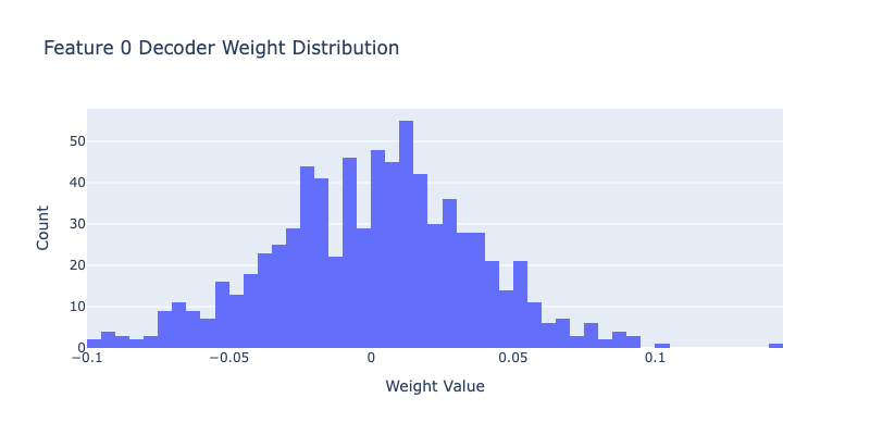
Let’s look at the decoder weights to understand what each feature represents. The decoder weights tell us how each feature contributes to the original activation.
1
2
3
4
5
6
7
8
9
10
11
12
13
14
15
16
17
18
19
20
21
22
23
24
25
26
27
28
29
30
31
32
33
34
35
36
37
38
39
40
41
42
43
44
45
46
47
48
49
50
def visualize_feature_decoder_weights(sae, feature_idx, n_top=20):
    """
    Visualize the decoder weights for a specific feature.
    Shows which directions in activation space this feature represents.

    Args:
        sae: Trained SparseAutoencoder
        feature_idx: Which feature to visualize
        n_top: Number of top weights to show
    """
    import IPython.display
    # Get decoder weights for this feature
    decoder_weights = sae.W_dec[:, feature_idx].detach().cpu().numpy()

    # Get top positive and negative weights
    top_pos_indices = np.argsort(decoder_weights)[-n_top:]
    top_neg_indices = np.argsort(decoder_weights)[:n_top]

    print(f"Feature {feature_idx} decoder weights:")
    print(f"\nTop {n_top} positive:")
    for idx in reversed(top_pos_indices):
        print(f"  Dimension {idx}: {decoder_weights[idx]:.4f}")

    print(f"\nTop {n_top} negative:")
    for idx in top_neg_indices:
        print(f"  Dimension {idx}: {decoder_weights[idx]:.4f}")

    # Plot histogram
    fig = go.Figure()
    fig.add_trace(go.Histogram(
        x=decoder_weights,
        nbinsx=50,
        name='Decoder Weights'
    ))

    fig.update_layout(
        title=f"Feature {feature_idx} Decoder Weight Distribution",
        xaxis_title="Weight Value",
        yaxis_title="Count",
        width=800,
        height=400
    )

    IPython.display.display(fig)

# Visualize a few features
print("Visualizing some learned features...\n")
for feature_idx in [0, 1000]:
    visualize_feature_decoder_weights(sae, feature_idx)
    print("\n" + "="*80 + "\n")
1
2
3
4
5
6
7
8
9
10
11
12
13
14
15
16
17
18
19
20
21
22
23
24
25
26
27
28
29
30
31
32
33
34
35
36
37
38
39
40
41
42
43
44
45
46
47
Visualizing some learned features...

Feature 0 decoder weights:

Top 20 positive:
  Dimension 481: 0.1429
  Dimension 521: 0.1003
  Dimension 107: 0.0948
  Dimension 155: 0.0912
  Dimension 550: 0.0906
  Dimension 127: 0.0890
  Dimension 498: 0.0880
  Dimension 440: 0.0873
  Dimension 94: 0.0859
  Dimension 3: 0.0843
  Dimension 716: 0.0819
  Dimension 216: 0.0793
  Dimension 573: 0.0792
  Dimension 609: 0.0788
  Dimension 285: 0.0769
  Dimension 447: 0.0768
  Dimension 270: 0.0760
  Dimension 513: 0.0716
  Dimension 13: 0.0708
  Dimension 448: 0.0701

Top 20 negative:
  Dimension 11: -0.0964
  Dimension 401: -0.0961
  Dimension 750: -0.0941
  Dimension 218: -0.0911
  Dimension 393: -0.0910
  Dimension 593: -0.0908
  Dimension 310: -0.0896
  Dimension 675: -0.0879
  Dimension 148: -0.0878
  Dimension 721: -0.0820
  Dimension 701: -0.0801
  Dimension 403: -0.0789
  Dimension 723: -0.0785
  Dimension 522: -0.0763
  Dimension 758: -0.0738
  Dimension 743: -0.0734
  Dimension 761: -0.0727
  Dimension 36: -0.0725
  Dimension 241: -0.0722
  Dimension 615: -0.0716
1
2
3
4
5
6
7
8
9
10
11
12
13
14
15
16
17
18
19
20
21
22
23
24
25
26
27
28
29
30
31
32
33
34
35
36
37
38
39
40
41
42
43
44
45
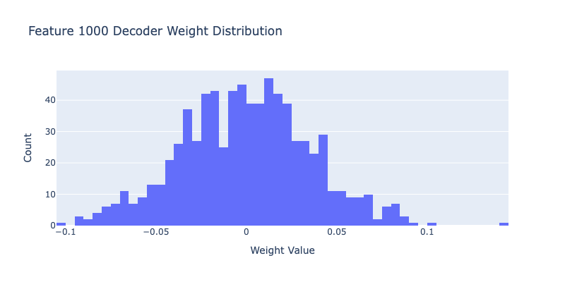
Feature 1000 decoder weights:
Top 20 positive:
Dimension 497: 0.1441
Dimension 577: 0.1001
Dimension 511: 0.0910
Dimension 527: 0.0897
Dimension 537: 0.0895
Dimension 279: 0.0875
Dimension 513: 0.0844
Dimension 602: 0.0836
Dimension 46: 0.0830
Dimension 460: 0.0827
Dimension 598: 0.0807
Dimension 763: 0.0803
Dimension 590: 0.0803
Dimension 38: 0.0798
Dimension 177: 0.0781
Dimension 224: 0.0778
Dimension 412: 0.0768
Dimension 450: 0.0765
Dimension 708: 0.0750
Dimension 767: 0.0730
Top 20 negative:
Dimension 737: -0.1044
Dimension 383: -0.0945
Dimension 374: -0.0942
Dimension 502: -0.0901
Dimension 281: -0.0866
Dimension 401: -0.0857
Dimension 748: -0.0847
Dimension 9: -0.0842
Dimension 444: -0.0841
Dimension 370: -0.0821
Dimension 367: -0.0800
Dimension 229: -0.0800
Dimension 2: -0.0788
Dimension 510: -0.0786
Dimension 208: -0.0782
Dimension 681: -0.0774
Dimension 409: -0.0743
Dimension 174: -0.0739
Dimension 373: -0.0726
Dimension 14: -0.0724
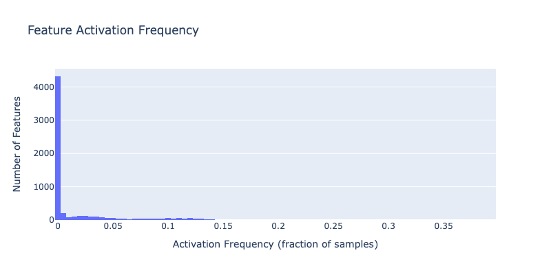
Dead Features Analysis
One challenge with SAEs is “dead features”. These are features that never activate. Let’s check how many of our features are actually being used.
1
2
3
4
5
6
7
8
9
10
11
12
13
14
15
16
17
18
19
20
21
22
23
24
25
26
27
28
29
30
31
32
33
34
35
36
37
38
39
40
41
42
43
44
45
46
47
48
49
50
51
52
53
54
55
56
def analyze_feature_usage(sae, dataloader, device='cuda'):
    """
    Analyze which features activate and how often.

    Args:
        sae: Trained SparseAutoencoder
        dataloader: DataLoader with activation data
        device: Device to run on

    Returns:
        feature_counts: How many times each feature activated
        feature_avg_activation: Average activation value per feature
    """
    sae.eval()

    feature_counts = torch.zeros(sae.cfg.d_hidden).to(device)
    feature_sums = torch.zeros(sae.cfg.d_hidden).to(device)
    total_samples = 0

    with torch.no_grad():
        for batch in tqdm(dataloader, desc="Analyzing feature usage"):
            batch = batch.to(device)

            # Encode
            features = sae.encode(batch)

            # Count active features
            feature_counts += (features > 0).float().sum(dim=0)

            # Sum activation values
            feature_sums += features.sum(dim=0)

            total_samples += batch.shape[0]

    # Compute statistics
    feature_frequency = feature_counts / total_samples
    feature_avg_activation = feature_sums / total_samples

    return feature_frequency.cpu(), feature_avg_activation.cpu()

print("Analyzing feature usage...\n")
feature_freq, feature_avg = analyze_feature_usage(sae, dataloader, device)

# Statistics
n_dead = (feature_freq == 0).sum().item()
n_alive = (feature_freq > 0).sum().item()

print(f"Feature usage statistics:")
print(f"  Total features: {cfg.d_hidden}")
print(f"  Active features: {n_alive} ({100*n_alive/cfg.d_hidden:.1f}%)")
print(f"  Dead features: {n_dead} ({100*n_dead/cfg.d_hidden:.1f}%)")
print(f"\nActivation frequency:")
print(f"  Mean: {feature_freq.mean():.4f}")
print(f"  Median: {feature_freq.median():.4f}")
print(f"  Max: {feature_freq.max():.4f}")
1
2
3
4
5
6
7
8
9
10
11
12
13
14
15
16
17
Analyzing feature usage...


Analyzing feature usage:   0%|          | 0/5268 [00:00<?, ?it/s]


Feature usage statistics:
  Total features: 6144
  Active features: 4180 (68.0%)
  Dead features: 1964 (32.0%)

Activation frequency:
  Mean: 0.0169
  Median: 0.0001
  Max: 0.3973
1
2
3
4
5
6
7
8
9
10
11
12
13
14
15
16
17
18
19
20
21
22
23
24
25
26
27
28
29
30
31
32
33
34
# Visualize feature usage
import IPython.display

fig = go.Figure()

fig.add_trace(go.Histogram(
    x=feature_freq.numpy(),
    nbinsx=100,
    name='Feature Frequency'
))

fig.update_layout(
    title="Feature Activation Frequency",
    xaxis_title="Activation Frequency (fraction of samples)",
    yaxis_title="Number of Features",
    width=800,
    height=400
)

IPython.display.display(fig)

# Show most and least frequent features
print("\nMost frequent features:")
top_features = torch.topk(feature_freq, 10)
for i, (freq, idx) in enumerate(zip(top_features.values, top_features.indices)):
    print(f"  {i+1}. Feature {idx.item()}: {freq.item()*100:.2f}% of samples")

print("\nLeast frequent (but alive) features:")
alive_freq = feature_freq[feature_freq > 0]
alive_indices = torch.where(feature_freq > 0)[0]
bottom_features = torch.topk(alive_freq, 10, largest=False)
for i, (freq, idx_in_alive) in enumerate(zip(bottom_features.values, bottom_features.indices)):
    actual_idx = alive_indices[idx_in_alive]
    print(f"  {i+1}. Feature {actual_idx.item()}: {freq.item()*100:.4f}% of samples")
1
2
3
4
5
6
7
8
9
10
11
12
13
14
15
16
17
18
19
20
21
22
23
Most frequent features:
  1. Feature 4656: 39.73% of samples
  2. Feature 5217: 39.09% of samples
  3. Feature 3808: 35.90% of samples
  4. Feature 2500: 24.65% of samples
  5. Feature 2902: 22.52% of samples
  6. Feature 5072: 22.03% of samples
  7. Feature 1123: 19.58% of samples
  8. Feature 615: 18.70% of samples
  9. Feature 1445: 18.40% of samples
  10. Feature 399: 17.05% of samples

Least frequent (but alive) features:
  1. Feature 23: 0.0001% of samples
  2. Feature 41: 0.0001% of samples
  3. Feature 140: 0.0001% of samples
  4. Feature 123: 0.0001% of samples
  5. Feature 191: 0.0001% of samples
  6. Feature 278: 0.0001% of samples
  7. Feature 360: 0.0001% of samples
  8. Feature 511: 0.0001% of samples
  9. Feature 313: 0.0001% of samples
  10. Feature 114: 0.0001% of samples
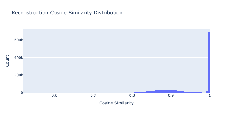
Reconstruction Quality
Let’s evaluate how well our SAE reconstructs the original activations. Good reconstruction means we’re not losing important information.
1
2
3
4
5
6
7
8
9
10
11
12
13
14
15
16
17
18
19
20
21
22
23
24
25
26
27
28
29
30
31
32
33
34
35
36
37
38
39
40
41
42
43
44
45
46
47
48
49
50
51
52
53
54
55
56
57
58
def evaluate_reconstruction(sae, dataloader, device='cuda'):
    """
    Evaluate reconstruction quality on a dataset.

    Args:
        sae: Trained SparseAutoencoder
        dataloader: DataLoader with activation data
        device: Device to run on

    Returns:
        metrics: Dictionary of reconstruction metrics
    """
    sae.eval()

    total_mse = 0
    total_mae = 0
    total_samples = 0
    cosine_sims = []

    with torch.no_grad():
        for batch in tqdm(dataloader, desc="Evaluating reconstruction"):
            batch = batch.to(device)

            # Forward pass
            x_recon, _ = sae(batch)

            # MSE
            mse = (batch - x_recon).pow(2).sum()
            total_mse += mse.item()

            # MAE
            mae = (batch - x_recon).abs().sum()
            total_mae += mae.item()

            # Cosine similarity
            cos_sim = F.cosine_similarity(batch, x_recon, dim=-1)
            cosine_sims.append(cos_sim)

            total_samples += batch.shape[0]

    # Compute averages
    cosine_sims = torch.cat(cosine_sims)

    metrics = {
        'mse': total_mse / total_samples,
        'mae': total_mae / total_samples,
        'cosine_sim_mean': cosine_sims.mean().item(),
        'cosine_sim_std': cosine_sims.std().item(),
    }

    return metrics, cosine_sims

print("Evaluating reconstruction quality...\n")
recon_metrics, cosine_sims = evaluate_reconstruction(sae, dataloader, device)

print(f"Reconstruction metrics:")
for k, v in recon_metrics.items():
    print(f"  {k}: {v:.6f}")
1
2
3
4
5
6
7
8
9
10
11
12
13
Evaluating reconstruction quality...


Evaluating reconstruction:   0%|          | 0/5268 [00:00<?, ?it/s]


Reconstruction metrics:
  mse: 49.943157
  mae: 115.925607
  cosine_sim_mean: 0.945239
  cosine_sim_std: 0.063504
1
2
3
4
5
6
7
8
9
10
11
12
13
14
15
16
17
18
# Visualize cosine similarities
fig = go.Figure()

fig.add_trace(go.Histogram(
    x=cosine_sims.cpu().numpy(),
    nbinsx=100,
    name='Cosine Similarity'
))

fig.update_layout(
    title="Reconstruction Cosine Similarity Distribution",
    xaxis_title="Cosine Similarity",
    yaxis_title="Count",
    width=800,
    height=400
)

IPython.display.display(fig)
1
2
3
4
5
6
7
8
9
10
11
12
13
14
15
16
17
18
19
20
21
22
23
24
25
26
27
28
29
30
31
32
33
34
35
36
37
38
39
40
def find_top_features(sae, dataloader, n=10):
    """Find features with good activation patterns"""
    sae.eval()

    feature_counts = torch.zeros(sae.cfg.d_hidden, device=device)
    feature_sums = torch.zeros(sae.cfg.d_hidden, device=device)
    total_samples = 0

    with torch.no_grad():
        for batch in dataloader:
            batch = batch.to(device)
            _, features = sae(batch)

            active = (features > 0).float()
            feature_counts += active.sum(dim=0)
            feature_sums += features.sum(dim=0)
            total_samples += len(batch)

    # Metrics
    freq = (feature_counts / total_samples).cpu().numpy()
    mean_act = (feature_sums / (feature_counts + 1e-8)).cpu().numpy()

    # Score: want medium frequency (1-10%), high magnitude
    freq_score = 1.0 - np.abs(freq - 0.05) / 0.05
    freq_score = np.clip(freq_score, 0, 1)

    mag_score = (mean_act - mean_act.min()) / (mean_act.max() - mean_act.min() + 1e-8)
    score = freq_score * mag_score

    top_idx = np.argsort(score)[-n:][::-1]

    return top_idx, freq, mean_act

print("Finding interesting features...")
interesting_features, freq, mean_act = find_top_features(sae, dataloader, n=10)

print(f"\n Top 10 Interesting Features: {interesting_features.tolist()}")
print("\nStatistics:")
for feat in interesting_features[:5]:
    print(f"  Feature {feat}: freq={freq[feat]:.3f}, magnitude={mean_act[feat]:.3f}")
1
2
3
4
5
6
7
8
9
10
Finding interesting features...

Top 10 Interesting Features: [3249, 3364, 2515, 5111, 1349, 2, 6126, 5127, 4879, 3070]

Statistics:
  Feature 3249: freq=0.052, magnitude=1.203
  Feature 3364: freq=0.017, magnitude=2.816
  Feature 2515: freq=0.045, magnitude=0.966
  Feature 5111: freq=0.048, magnitude=0.877
  Feature 1349: freq=0.033, magnitude=1.205
1
2
3
4
5
6
7
8
9
10
11
12
13
14
15
16
17
18
19
20
21
22
23
24
25
26
27
28
29
30
31
32
33
34
35
36
37
38
39
40
41
42
43
44
45
46
47
48
def find_activating_features_for_text(
    text: str,
    model,
    sae,
    layer_idx: int = 6,
    min_activation: float = 0.5,
    top_k: int = 10
):
    """
    Find features that ACTUALLY activate strongly on this specific text.

    Returns features sorted by their max activation on this text.
    """
    # Get token-level features
    tokens = model.to_tokens(text, prepend_bos=True)
    token_strs = model.to_str_tokens(text, prepend_bos=True)

    with torch.no_grad():
        _, cache = model.run_with_cache(tokens)
        acts = cache[f"blocks.{layer_idx}.hook_mlp_out"][0]
        _, features = sae(acts)

    features_np = features.cpu().numpy()  # Shape: [seq_len, n_features]

    # Find max activation for each feature across all tokens
    max_activations = features_np.max(axis=0)  # Shape: [n_features]

    # Filter features that actually activate
    active_features = np.where(max_activations > min_activation)[0]

    if len(active_features) == 0:
        print(f"Warning: No features activated above {min_activation}")
        print(f"   Lowering threshold to find ANY activating features...")
        min_activation = max_activations.max() * 0.1  # 10% of max
        active_features = np.where(max_activations > min_activation)[0]

    # Sort by activation strength
    sorted_indices = np.argsort(max_activations[active_features])[::-1]
    top_features = active_features[sorted_indices[:top_k]]

    print(f"\nFound {len(active_features)} features activating above {min_activation:.2f}")
    print(f"Top {len(top_features)} features by max activation:")
    for i, feat_idx in enumerate(top_features[:5], 1):
        max_act = max_activations[feat_idx]
        num_tokens = (features_np[:, feat_idx] > 0.1).sum()
        print(f"   {i}. Feature {feat_idx}: max={max_act:.3f}, active on {num_tokens}/{len(token_strs)} tokens")

    return top_features, token_strs, features_np
1
2
3
4
5
6
7
8
9
10
11
12
13
14
15
16
17
18
19
20
21
22
23
24
25
26
27
28
29
30
31
32
33
34
35
36
37
38
39
40
41
42
43
44
45
46
47
48
49
50
51
52
53
54
55
56
57
58
59
60
61
62
63
64
65
66
67
68
69
70
71
72
73
74
75
76
77
78
79
80
81
82
83
84
85
86
87
88
89
90
91
92
93
94
95
96
97
98
99
100
101
102
103
104
105
106
107
108
109
110
111
112
113
114
115
116
117
118
119
120
121
122
123
124
125
126
127
128
129
130
131
132
133
134
135
136
137
138
139
140
141
142
143
144
145
def create_visualization(
    text: str,
    model,
    sae,
    layer_idx: int = 6,
    n_features: int = 4,
    min_activation: float = 0.5
):
    """
    Create visualization using features that ACTUALLY activate on this text.
    """

    print(f"Analyzing text: '{text}'")
    print("=" * 80)

    # Step 1: Find features that activate on THIS text
    top_features, token_strs, features_np = find_activating_features_for_text(
        text, model, sae, layer_idx, min_activation, n_features
    )

    if len(top_features) == 0:
        print("ERROR: No features found! Try a different text or check your SAE.")
        return

    # Limit to requested number
    features_to_show = top_features[:n_features]

    # Step 2: Create the visualization
    fig = make_subplots(
        rows=len(features_to_show) + 1,
        cols=1,
        subplot_titles=['Feature Activation Heatmap'] +
                       [f'Feature {f} (max: {features_np[:, f].max():.2f})' for f in features_to_show],
        vertical_spacing=0.04,
        row_heights=[0.25] + [0.75/len(features_to_show)] * len(features_to_show)
    )

    # Plot 1: Heatmap
    selected = features_np[:, features_to_show]

    fig.add_trace(
        go.Heatmap(
            z=selected.T,
            x=token_strs,
            y=[f'F{f}' for f in features_to_show],
            colorscale='Viridis',
            showscale=True,
            colorbar=dict(
                title="Activation",
                len=0.25,
                y=0.88,
                x=1.02
            ),
            hovertemplate='Token: %{x}<br>%{y}<br>Activation: %{z:.3f}<extra></extra>'
        ),
        row=1, col=1
    )

    # Plot 2: Individual feature bars
    colors = ['rgb(99,110,250)', 'rgb(239,85,59)', 'rgb(0,204,150)', 'rgb(255,161,90)']

    for i, feat_idx in enumerate(features_to_show, start=2):
        feat_acts = features_np[:, feat_idx]
        max_act = feat_acts.max()

        # Color gradient based on activation strength
        if max_act > 0:
            intensities = feat_acts / max_act
        else:
            intensities = np.zeros_like(feat_acts)

        color_base = colors[i-2] if i-2 < len(colors) else 'rgb(150,150,150)'
        bar_colors = [
            f'rgba({color_base[4:-1]}, {0.2 + 0.8 * intensity})'
            for intensity in intensities
        ]

        fig.add_trace(
            go.Bar(
                x=token_strs,
                y=feat_acts,
                marker=dict(
                    color=bar_colors,
                    line=dict(color=color_base, width=1.5)
                ),
                showlegend=False,
                hovertemplate='Token: %{x}<br>Activation: %{y:.3f}<extra></extra>'
            ),
            row=i, col=1
        )

        # Add threshold line (mean + std)
        threshold = feat_acts.mean() + feat_acts.std()
        fig.add_hline(
            y=threshold,
            line=dict(color='red', dash='dash', width=1),
            row=i, col=1
        )

    # Update layout
    fig.update_layout(
        height=200 * (len(features_to_show) + 1),
        title=dict(
            text=f"<b>Feature Activation Analysis</b><br><sub>{text[:100]}...</sub>",
            x=0.5,
            xanchor='center'
        ),
        template='plotly_white',
        showlegend=False
    )

    # Update axes
    for i in range(1, len(features_to_show) + 2):
        fig.update_xaxes(
            tickangle=-45,
            tickfont=dict(size=9),
            row=i, col=1
        )
        fig.update_yaxes(
            title_text="Activation",
            row=i, col=1
        )

    fig.show()

    # Print interpretation
    print("\n" + "=" * 80)
    print("INTERPRETATION")
    print("=" * 80)

    for feat_idx in features_to_show:
        feat_acts = features_np[:, feat_idx]
        top_token_idx = np.argmax(feat_acts)

        # Find all highly active tokens
        threshold = feat_acts.mean() + feat_acts.std()
        active_tokens = [(i, token_strs[i], feat_acts[i])
                        for i in range(len(token_strs))
                        if feat_acts[i] > threshold]

        print(f"\n Feature {feat_idx}")
        print(f"   Max activation: {feat_acts.max():.3f} at token '{token_strs[top_token_idx]}'")
        print(f"   Highly active tokens: {', '.join([f'{tok} ({act:.2f})' for _, tok, act in active_tokens])}")
1
2
3
4
5
6
7
create_visualization(
        "The stock market reacted very poorly to the news",
        model,
        loaded_sae,
        n_features=10,
        min_activation=0.5  # Adjust this if needed
    )
1
2
3
4
5
6
7
8
9
10
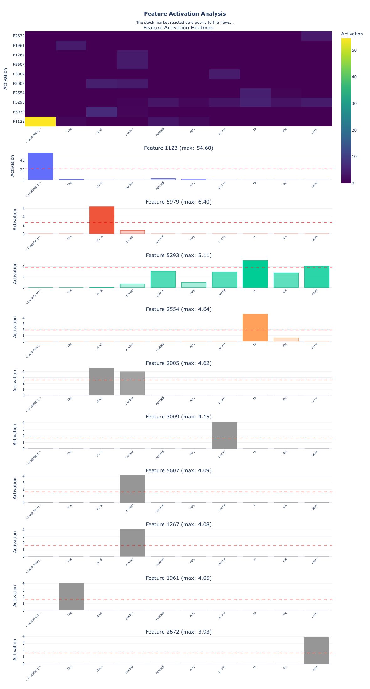
Analyzing text: 'The stock market reacted very poorly to the news'
================================================================================
Found 430 features activating above 0.50
Top 10 features by max activation:
1. Feature 1123: max=54.601, active on 4/10 tokens
2. Feature 5979: max=6.405, active on 2/10 tokens
3. Feature 5293: max=5.115, active on 7/10 tokens
4. Feature 2554: max=4.638, active on 2/10 tokens
5. Feature 2005: max=4.619, active on 2/10 tokens
1
2
3
4
5
6
7
8
9
10
11
12
13
14
15
16
17
18
19
20
21
22
23
24
25
26
27
28
29
30
31
32
33
34
35
36
37
38
39
40
41
42
43
================================================================================
INTERPRETATION
================================================================================

 Feature 1123
   Max activation: 54.601 at token '<|endoftext|>'
   Highly active tokens: <|endoftext|> (54.60)

 Feature 5979
   Max activation: 6.405 at token ' stock'
   Highly active tokens:  stock (6.40)

 Feature 5293
   Max activation: 5.115 at token ' to'
   Highly active tokens:  to (5.11),  news (4.04)

 Feature 2554
   Max activation: 4.638 at token ' to'
   Highly active tokens:  to (4.64)

 Feature 2005
   Max activation: 4.619 at token ' stock'
   Highly active tokens:  stock (4.62),  market (3.97)

 Feature 3009
   Max activation: 4.149 at token ' poorly'
   Highly active tokens:  poorly (4.15)

 Feature 5607
   Max activation: 4.090 at token ' market'
   Highly active tokens:  market (4.09)

 Feature 1267
   Max activation: 4.078 at token ' market'
   Highly active tokens:  market (4.08)

 Feature 1961
   Max activation: 4.053 at token 'The'
   Highly active tokens: The (4.05)

 Feature 2672
   Max activation: 3.930 at token ' news'
   Highly active tokens:  news (3.93)
Some key things to notice in this analysis:
1. Hierarchical Feature Types The features naturally organize into different levels:
- Positional: Feature 1123 (54.60) fires exclusively on
<|endoftext|>, marking sequence boundaries - Domain-specific: Features 5979, 2005, 5607, 1267 all activate on financial terms (“stock”, “market”)
- Semantic: Feature 3009 detects “poorly” (negative sentiment), Feature 2672 detects “news” (information source)
- Syntactic: Feature 1961 captures the determiner “The”, Feature 2554 the preposition “to”
2. Multiple Features Per Token Notice how “stock” activates two features (5979 & 2005), and “market” activates two features (5607 & 1267). This is the SAE decomposing polysemy the same word can activate different features depending on context. One might represent “stock” in financial contexts, another “stock” as part of the phrase “stock market.”
3. Multi-Token Features
Feature 5293 spreads across “to” and “news” as it’s not just detecting individual words but capturing relationships between them. This shows features can represent multi-token patterns.
4. Varying Importance Activation strengths range from 3.93 to 54.60, suggesting different features contribute different amounts to the representation. The beginning-of-sequence feature fires 10x stronger than domain features, indicating its foundational role in processing.
Key Takeaways
Awesome, we have built a Sparse Autoencoder from scratch and trained it on real neural network activations. Let’s recap what we learned:
The Problem: Superposition
- Neural networks store more features than they have dimensions
- Features are “compressed” into overlapping directions (superposition)
- This makes individual neurons uninterpretable
- Sparsity allows this compression to work with minimal interference
The Solution: Sparse Autoencoders
- Expand to high-dimensional space (e.g., 768 → 6,144)
- Enforce sparsity through L1 penalty (only few features active)
- Reconstruct original activations accurately
- Result: Each dimension corresponds to an interpretable feature
Architecture Details
- Encoder: Linear projection + ReLU
- ReLU creates hard zeros (true sparsity)
- Pre-bias subtraction centers the data
- Decoder: Linear projection back to original space
- Normalized columns for training stability
- Learned bias captures mean activation
- Loss Function: Reconstruction + Sparsity
- MSE loss ensures accurate reconstruction
- L1 penalty encourages sparse activations
- λ (lambda) controls the trade-off
What We Found
- Sparsity: Only a small fraction of features active per sample
- Reconstruction: High cosine similarity to original activations
- Dead features: Some features never activate (common issue)
- Feature diversity: Different features for different patterns
Practical Insights
- Expansion factor: 8x to 32x typical (more = more features, slower training)
- Sparsity coefficient: Tune λ to balance interpretation vs reconstruction
- Layer choice: Middle layers often have most interesting features
- Data quantity: More data = better features (we used minimal for demo)
- Dead features: Can be reduced with techniques like:
- Higher learning rate
- L2 regularization
- Auxiliary losses
- Better initialization
Applications of SAEs
Sparse Autoencoders are powerful tools for:
1. Mechanistic Interpretability
- Circuit discovery: Find which features connect to others
- Feature attribution: Trace model decisions to specific features
- Failure mode analysis: Identify features responsible for errors
2. Model Steering
- Feature manipulation: Amplify/suppress specific features
- Controlled generation: Activate features for desired outputs
- Bias mitigation: Identify and remove unwanted features
3. Safety and Alignment
- Deception detection: Find features related to misleading behavior
- Goal representation: Understand what the model is optimizing for
- Monitoring: Track dangerous capabilities through features
Limitations and Future Directions
Current Limitations
- Dead features: Not all learned features are used
- Polysemanticity: Some features still respond to multiple concepts
- Scale: Training SAEs on large models is computationally expensive
- Verification: Hard to verify that features are truly monosemantic
Active Research
- Better architectures: Gated SAEs, TopK SAEs, VAE-style SAEs
- Training improvements: Curriculum learning, auxiliary losses
- Scaling: Efficient training on billion-parameter models
- Evaluation: Better metrics for feature quality
- Applications: Using SAEs for model editing and steering
Resources and References
Papers
- Toy Models of Superposition - Anthropic’s foundational work
- Towards Monosemanticity - Anthropic’s SAE work
- Scaling Monosemanticity - Scaling to larger models
- Sparse Autoencoders Find Highly Interpretable Features - Academic perspective
Code and Tools
- SAELens - Library for training and analyzing SAEs
- TransformerLens - Clean transformers with hooks
- Neuronpedia - Interactive visualization of SAE features